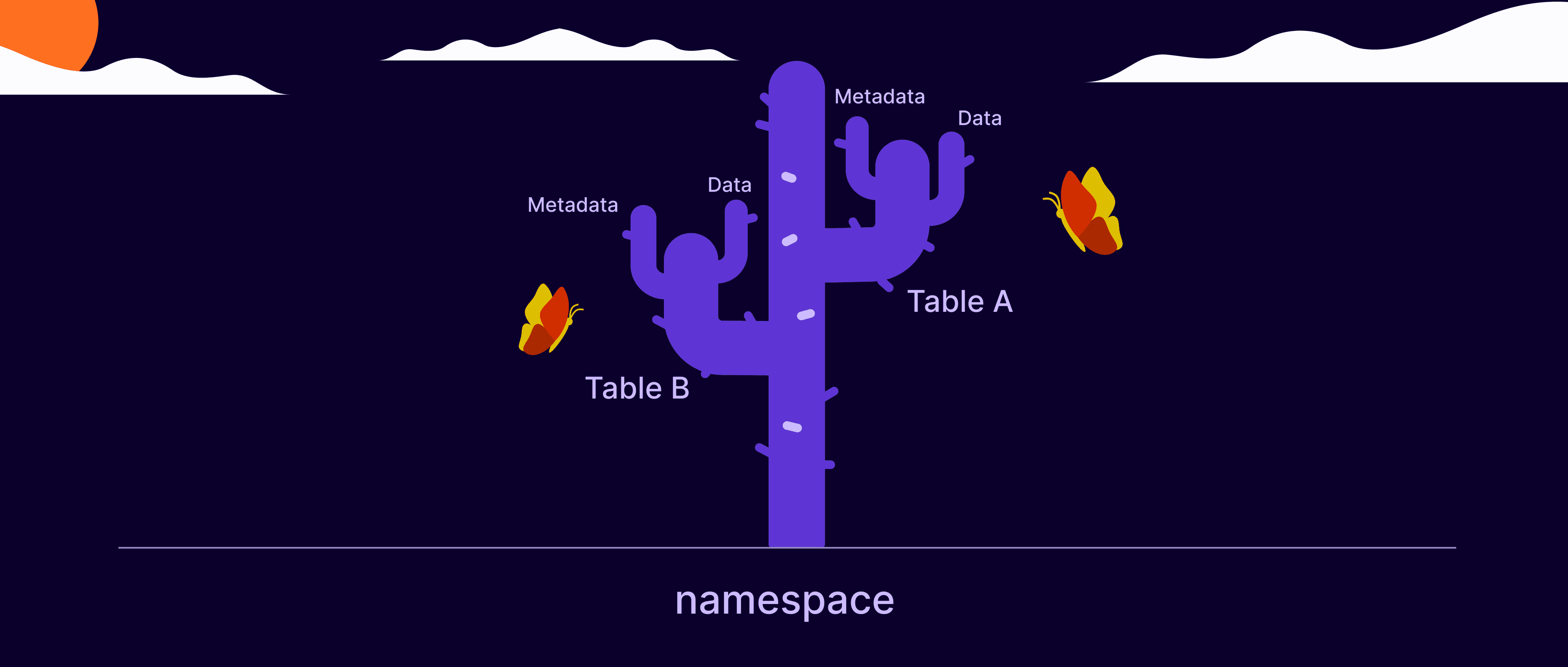
How many cacti does it take to make an Iceberg?

The answer is "as many as you have namespaces," and we will explain why in a second.

All six posts of this 6-part series are now available:

Part 1: Building Open, Multi-Engine Lakehouse with S3 and Python

Part 2: How Iceberg stores table data and metadata

Part 3: Picking Snowflake Open Catalog as a managed Iceberg catalog

Part 4: How to create S3 buckets to store your lakehouse

Part 5: How to set up a managed Iceberg catalog using Snowflake Open Catalog

Part 6: How to write Iceberg tables using PyArrow and analyze them using Polars

But first, let's clarify what icebergs we are talking about. Apache Iceberg is a standard for defining tables on top of open file formats like Parquet and cloud storage like S3. 

If you came here after reading our post about building open lakehouses just by using Python and S3, you already know that Iceberg is being quickly adopted as the new format for so-called lakehouses — Data Lakes that can act as Data Warehouses by allowing users to query their contents as tables.

An Iceberg lakehouse has N namespaces; each namespace can have M tables, and these tables store their data in 2 folders: "data" and "metadata" containing many files. If a namespace can be thought of as a proud cactus of the Saguaros species, then tables and folders of the tables are the branches of the said cactus and the individual files - the thorns. A complete Iceberg lakehouse is, therefore, a forest of cacti. 

Now that the mystery is solved, let's learn more about Iceberg. 

In this post, we will provide you with the tools for exploring Iceberg's table data and metadata storage so that you can better understand the performance and concurrency challenges and solutions of operating a multi-engine, open lakehouse. 

If you are comfortable with command line tools like the AWS CLI, we recommend downloading the sample Iceberg files we prepared for you and following this exploration on your development machine.

How to configure your local dev environment for exploring Iceberg storage

Skip this step if you can run the following command without errors!

aws s3 ls

This step is optional if you already have a local development environment setup that allows you to inspect cloud object storage in AWS, but for those of you who are new to this, we recommend doing two things:

1. Sign up for a free AWS account

2. Set up a "data engineer" user and user group

3. Set up the AWS CLI (command line interface) on your development machine (e.g., your laptop)

   
   

Set up a “data engineer” user and group

We recommend this step so that you don't always have to use your "root" AWS account (this is a security risk).

1. Login to AWS Management Console as the "root" user

2. Go to IAM

3. In the side-bar menu, under Access Management, pick "Users"

4. Click on "Create user"

5. Give this user a name (we will use "dataeng1" here)

6. On the "Set permissions" page, select "Add user to group" and select "Create user group"

7. In the "Create user group" page, give the group a name like "DataEngineersGroup" and select the "PowerUserAccess" policy

8. Finalize by clicking on "Create user"

Once you create the user, get its access keys:

1. Open the user

2. Switch to the Security credentials tab

3. Under "Access keys", click on Create access key

4. Under "Use case", pick "Command Line Interface"

5. Once you create the access key and the associated secret access key, save them somewhere secure because you will need them for the next step

(Note that we are using Long-Term credentials here, which AWS is trying to discourage when accessing production data. Since we are building a development environment, using the long-term credentials is OK.)

Set up the AWS CLI locally on your dev box

Follow the instructions on this page to install the AWS CLI.

You can now create the config and credentials files where you will place your user's access keys.

mkdir ~/.aws
cd .aws
touch config
touch

Create a profile for the user "dataeng1" in the config file.

In the credentials file, save the user's access keys.

You can set the active profile by setting the AWS_PROFILE shell variable.

export AWS_PROFILE

From here on, when you call the AWS CLI, it will use the credentials of the active profile. 

Try this command to see if you can access our sample set of lakehouse files. These files comprise the state of one of our sample lakehouses as of mid-November 2024.

aws s3 ls s3://mango-public-data/lakehouse-snapshots/peach-lake --recursive

If you get a list of several files, you are all set!

Learning what’s inside an Iceberg Lakehouse

We published several snapshots of a sample Iceberg lakehouse on a public read-only bucket in S3 (s3://mango-public-data/lakehouse-snapshots/peach-lake). 

We will use these snapshots, which consist of folders and files in JSON, Avro, and Parquet format, to walk you through the contents of an Iceberg lakehouse.

Let's download our first snapshot (stored in the "s0" subfolder) locally.

# go to a temp folder
cd /tmp

# download the s0 folder containing a snapshot of a sample lakehouse
aws s3 sync s3://mango-public-data/lakehouse-snapshots/peach-lake/s0/ s0

Let's run a local ls command to list all the files that we downloaded.

# check that all files were downloaded
ls -R s0

default

s0/default:
japan_trade_stats_2017_2020

s0/default/japan_trade_stats_2017_2020:
data		metadata

s0/default/japan_trade_stats_2017_2020/data:
00000-0-b0823e8d-5894-4b67-ae80-0ff4a480e1c0.parquet	00000-2-b0823e8d-5894-4b67-ae80-0ff4a480e1c0.parquet
00000-1-b0823e8d-5894-4b67-ae80-0ff4a480e1c0.parquet

s0/default/japan_trade_stats_2017_2020/metadata:
00000-6ae8bff7-eb6b-4c09-92ad-9ff0a7e93062.metadata.json
00001-5d511f22-9819-47fd-a010-97d75a964dfd.metadata.json
b0823e8d-5894-4b67-ae80-0ff4a480e1c0-m0.avro
snap-1893044843699371523-0-b0823e8d-5894-4b67-ae80-0ff4a480e1c0.avro

You are in good shape if you got a similar output from the last command.

Let's explore how Iceberg stores data. Typically, in a data warehouse, you have multiple schemas; within each schema, you have several tables. Iceberg allows you to do that as well. Schemas are called namespaces in Iceberg and are stored in separate folders in S3. Each table of a namespace will reside in its separate folder under the namespace folder, and under the table's folder, there will be two subfolders: "data" and "metadata." The "data" and "metadata" folders will contain several JSON, Avro, and Parquet files. The “data” folder will contain data files, and the “metadata” folder will contain the metadata file, the manifest list files and the manifest files.

Metadata file

The most important file of a table is the *.metadata.json file. It is called the metadata file or the root file, and it contains the table schema and references to files containing the table's data. 

Whenever you change the schema of a table or add or remove rows to a table, you will create a new metadata file that will become the "current" one. Over time, you will see a bunch of *.metadata.json files under the "metadata" folder. Their names will differ in a sequence number - 00000, 00001, 00002, and so on - and the additional unique id. These files store different versions of the table metadata as you keep changing the table.

In our example, there are two metadata.json files (sequence numbers 00000 and 00001) in our "metadata" folder because to produce this snapshot, we made two operations on the table: we created it, and we executed an "append." 

Let's look inside the metadata file with the sequence number 00001. This metadata file contains the state of the table after several records were inserted into it. 

cd s0/default/japan_trade_stats_2017_2020/metadata
nano 00001-5d511f22-9819-47fd-a010-97d75a964dfd

Use your favorite text editor to look inside the file. If you are on a Mac and need help finding the folder where your files are located, type

open -a

The metadata.json file tracks where the table data is stored via an internal "snapshots" section. For example, in the table you downloaded, there is just one snapshot with sequence number 1. 

Contents of the Iceberg metadata file “00001-5d511f22-9819-47fd-a010-97d75a964dfd.metadata.json”

…
  "snapshots" : [ {
    "sequence-number" : 1,
    "snapshot-id" : 1893044843699371523,
    "timestamp-ms" : 1731442065673,
    "summary" : {
      "operation" : "append",
      "added-files-size" : "117464606",
      "added-data-files" : "3",
      "added-records" : "14897200",
      "total-data-files" : "3",
      "total-delete-files" : "0",
      "total-records" : "14897200",
      "total-files-size" : "117464606",
      "total-position-deletes" : "0",
      "total-equality-deletes" : "0"
    },
    "manifest-list" : "s3://peach-lake/default/japan_trade_stats_2017_2020/metadata/snap-1893044843699371523-0-b0823e8d-5894-4b67-ae80-0ff4a480e1c0.avro",
    "schema-id" : 0
  } ],
…

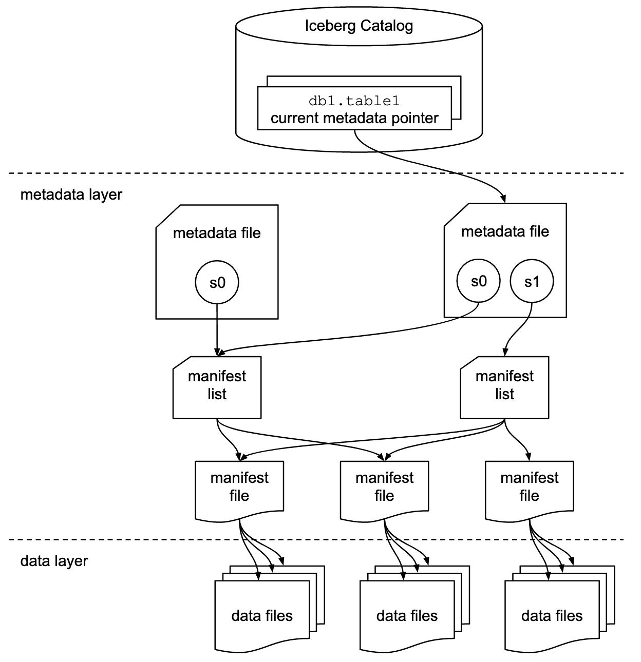
As we can see, this snapshot was created through an append operation, which added 3 data files containing about 14.89 million records. There is also a reference to another file called "manifest-list." The file name (snap-1893044843699371523-0-b0823e8d-5894-4b67-ae80-0ff4a480e1c0.avro) starts with the prefix "snap" and ends in the .avro extension. As we go through each of these sample files, you will see more and more references to other files stored in them. We are dealing here with a graph of references. 

This graph is best visualized in the following diagram, borrowed from the official Iceberg spec. The files we downloaded from S3 correspond to the left branch of this graph: a table with with just one snapshot.

Manifest list files (aka “Snapshot files”)

Why do we need these manifest lists, and what's stored there? Lists of manifests, of course! 

Before you hit us with something hard, let's understand how Iceberg organizes table data.

In the previous section, when looking at our metadata file, we encountered snapshot #1, which references the manifest list file "snap-1893044843699371523-0-b0823e8d-5894-4b67-ae80-0ff4a480e1c0.avro".

To look inside Avro files, pip-install the Avro package and run the avro cat command. 

pip install avro
avro cat

You could also use one of the online Avro viewers (e.g., Konbert) or VSCode plugins, but be careful uploading actual production data into the free services (uploading test data should be OK).

Contents of the manifest list file “snap-1893044843699371523-0-b0823e8d-5894-4b67-ae80-0ff4a480e1c0.avro”

{
	"manifest_path": "s3://peach-lake/default/japan_trade_stats_2017_2020/metadata/b0823e8d-5894-4b67-ae80-0ff4a480e1c0-m0.avro",
	"manifest_length": 6504,
	"partition_spec_id": 0,
	"content": 0,
	"sequence_number": 1,
	"min_sequence_number": 1,
	"added_snapshot_id": 1893044843699371523,
	"added_files_count": 3,
	"existing_files_count": 0,
	"deleted_files_count": 0,
	"added_rows_count": 14897200,
	"existing_rows_count": 0,
	"deleted_rows_count": 0,
	"partitions": [],
	"key_metadata": null
}

Our snap...avro manifest list file contains a very short list with just one record called a manifest.

This manifest is referenced in the "manifest_path" field and stored as an Avro file. In our case, this file's name is "b0823e8d-5894-4b67-ae80-0ff4a480e1c0-m0.avro". Notice the "m0" after the unique ID and before the file extension. It indicates that the file contains a manifest (distinguishing it from manifest lists stored in files with the prefix "snap").

Summary: There is precisely one "manifest list" file per logical snapshot, and these manifest lists track the snapshot of a table (both data and schema) at a particular moment in time.

Manifest files 

Let's continue down the Iceberg graph and look at our manifest file.

A manifest contains a list of "data" and "delete" files. Data files store the table's records at a particular snapshot. Delete files, however, store records deleted from data files (in some other databases, these are called deletion vectors). A table's data may reside in 1 to N data and deletion files. 

Unfortunately, we could not get the pip-installed avro command to process our manifest files. We could read the "manifest list" files without issues, but we could not read the "manifest" files.  

An exception in avro/schema.py, "IgnoredLogicalType: Unknown map, using array," and another one in json/encoder.py, "TypeError: Object of type bytes is not JSON serializable," kept causing trouble even after we upgraded to newer versions of Python and Avro. 

Luckily, Naveen Kumar included an example of a manifest file in his post, which we summarize below. 

Contents of an Iceberg manifest file

{
  "status": 1,
  "snapshot_id": {
    "long": 3854344042660880000
  },
  "sequence_number": null,
  "file_sequence_number": null,
  "data_file": {
    "content": 0,
    "file_path": "s3://<removed>/data/<removed>.parquet",
    "file_format": "PARQUET",
    "partition": {
      "category": {
        "string": "c1"
      }
    },
    "record_count": 1,
    "file_size_in_bytes": 881,
…

The “data_file” section of the manifest file points to our data files via the "file_path" field. The manifest file also has some useful statistics about the data files:

• column_sizes

• value_counts

• null_value_counts

• nan_value_counts

• lower_bounds

• upper_bounds

These stats allow the querying engine to do so-called pruning and decide which data files to read and not to read based on the parameters of a query.

Data files

With this, we reached the bottom layer of our Iceberg table graph - the "data" and "delete" files. 

Data files store table records. These files are usually in Parquet format, are named <uuid>.parquet, and are located in the "data" folder of the table's S3 folder. However, data files, by Iceberg spec, can also be in ORC or Avro formats.

Udaya Chathuranga has a great post on how this 4-level graph design enables fast read and write processing in Iceberg tables. This design, IMHO, was chosen to take advantage of the block storage capabilities of S3, Azure Storage, and GCS to implement transactional database storage for analytical workloads.   

Next Steps

If you liked our little exploration of Iceberg storage, follow us on Linkedin or sign up for our Substack newsletter to get notified when we publish the next post in this series. In that post, we will review available Iceberg catalog options and share why Snowflake's Open Catalog was a top choice (at least for now).

In our final post of the series, we will tie everything together and show how to use standard Python tools (PyArrow and Polars) to run data applications on top of an S3-based open lakehouse.